UAV Aerial Mapping for Crop Health Monitoring
AEROSPACE REMOTE SENSING PIPELINE
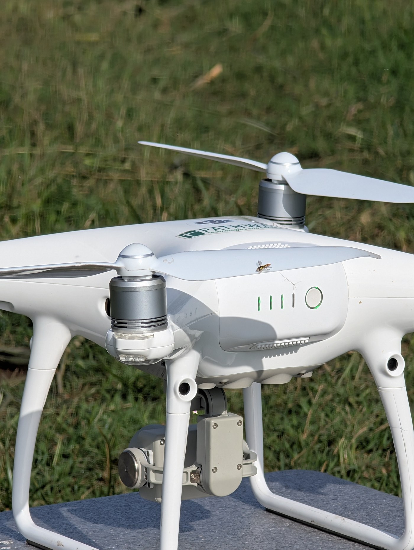
The DJI Phantom 4 Pro V2.0 UAV platform in the field.
Video autoplays muted. Use the player controls to unmute.
Overview
This was our final year project in the Department of Mechanical and Aerospace Engineering at Pulchowk Campus. We wanted to find out whether an ordinary RGB camera on a commercial drone can tell us how well a maize crop is doing on nitrogen. To test that, we flew a DJI Phantom 4 Pro V2.0 over an experimental maize field at the IAAS Rampur Campus in Chitwan, built orthomosaic maps of the field, calculated six vegetation indices from them, and compared the numbers with 240 SPAD chlorophyll readings taken by hand on the ground.
On top of that we wrote a Python pipeline that separates the maize canopy from soil, and trained a Random Forest model that classifies the canopy as nutrient sufficient or nutrient deficient. The whole workflow is shown in the flowchart below, from planning the flights to marking the deficient zones on a map.
The methodology was set up as a multi-stage process that joined UAV data collection, photogrammetric processing, vegetation index analysis in QGIS, machine learning classification and ground-truth validation. Each stage builds on the output of the one before it, so the pipeline runs from raw aerial images all the way to the location of nutrient sufficient and deficient zones in the field.
Background
Maize is the second most important staple crop in Nepal after rice, and it matters a lot for food security, rural livelihoods and farming that can last. It grows across many different regions and is a main source of food, animal feed and income for smallholder farmers. Even though the crop has a high yield potential, maize productivity in Nepal stays low compared with global standards, mostly because nutrients are not managed properly or in the right balance.
Earlier studies have shown that maize growth and yield depend strongly on how nutrients are supplied. Different combinations of organic and inorganic fertilizer give very different results, and tools such as analysis of variance (ANOVA) and regression are the usual way to test those differences. More recently, vegetation indices such as the Visible Atmospherically Resistant Index (VARI), Green Leaf Index (GLI), Triangular Greenness Index (TGI) and Normalized Green-Red Difference Index (NGRDI) have become a non-destructive way to judge crop vigor and nutrient status from canopy reflectance. Their use on maize under different nutrient conditions, especially in Nepal, is still limited.
In practice, most farmers still judge crop health by eye and by experience, which often misses early nutrient deficiencies and makes it hard to apply fertilizer at the right rate. That is the gap we wanted to work on: combining statistical methods with spectral indices to give a more precise, quantitative picture of how maize responds to different nutrient treatments.
Problem Statement
Traditional crop monitoring is slow, needs a lot of labor and does not work well over large areas. Multispectral sensors give accurate vegetation indices, but they are too expensive for most smallholder farmers. Low-cost RGB cameras on UAVs are a promising alternative, but the existing RGB approaches are inefficient because they depend on manual data collection and complicated post-processing, which limits their use for timely crop health monitoring.
This study therefore tries to build a solid mathematical relationship between RGB-derived vegetation indices (such as VARI) and the physiological status of the crop under different fertilization treatments, including urine-enriched biochar. The aim is a method that is cheap, scalable and non-destructive.
Objectives
Main objective: to assess the nutritional status of maize using UAV based RGB aerial imagery, by calculating and comparing several vegetation indices.
Specific objectives:
- To fly systematic UAV missions that capture high-resolution RGB images and to generate georeferenced orthomosaic maps
- To develop an image processing pipeline that segments the maize canopy and removes non-vegetation pixels
- To compute several RGB-derived vegetation indices from the masked canopy imagery and map how they are distributed across the experimental plots
- To measure the effect of six different nutrient treatments on crop chlorophyll content using SPAD-502 meter readings across four replications
Where It Can Be Used
- Early and accurate detection of maize nutrient deficiencies, so that action can be taken in time
- Site-specific nutrient application, which improves fertilizer use efficiency and productivity
- Lower labor and cost compared with traditional crop monitoring, since a UAV does the survey
- Reliable data for agricultural extension services and for policy decisions
- A framework that can be adapted to other crops and regions
Study Area and Experimental Design
Before any flying started, we prepared the field together with the Nepal Agricultural Research Council (NARC) and GeoKrishi. The experiment was carried out at the research farm of IAAS, Rampur Campus, Chitwan (213 m above sea level), where the climate is subtropical and well suited to maize. The land was ploughed several times to get a fine, even soil structure, crop residues and weeds were removed, the field was levelled and well-decomposed farmyard manure was applied.
The layout was a Randomized Complete Block Design (RCBD) with six treatments and four replications, giving 24 plots. Each plot measured 3 m by 3 m, with 1 m spacing between plots and blocks, and the crop geometry was 60 cm by 25 cm. Using RCBD makes it possible to separate the effect of the treatments from natural variation in the field, such as differences in soil. The six treatments ran from a control with no nitrogen up to different combinations of urea, biochar and organic nitrogen sources:
- T1: control, no nutrient
- T2: 100% RDN through urea
- T3: 100% RDN through urea plus biochar (1 t/ha)
- T4: 100% RDN through urea-enriched biochar
- T5: 50% RDN through urea and 50% N through cattle urine enriched biochar
- T6: 50% RDN through urea and 50% N through human urine enriched biochar
The recommended fertilizer dose was 180:60:60 kg N:P2O5:K2O per hectare. The nitrogen came from urea, with one-third (60 kg/ha) as a basal dose and the remaining two-thirds (120 kg/ha) split equally between the knee height and tasseling stages. Rampur Hybrid-12 maize was the test crop, sown at two seeds per hill and thinned to one plant at the V2 stage. All other agronomic practices were the same for every plot.
Equipment and Software
The hardware was a DJI Phantom 4 Pro V2.0 with its RGB imaging system, a SPAD chlorophyll meter for ground truth, a tablet running the flight apps, high-speed SD cards, a multi-battery charger and hub for field days, and a workstation for image processing.
We picked the Phantom 4 Pro V2.0 for its high-resolution camera and the OcuSync transmission system. It weighs 1375 g with battery and propellers, has a 350 mm diagonal size, resists wind up to 10 m/s and flies for about 30 minutes on a 5870 mAh battery. The camera has a 1-inch CMOS sensor with 20 effective megapixels, an 84 degree field of view (8.8 mm lens, 24 mm in 35 mm format), an aperture of f/2.8 to f/11 and a mechanical shutter from 8 s to 1/2000 s. It sits on a 3-axis gimbal, and positioning uses GPS and GLONASS.
For software we used DroneDeploy for mission planning and orthomosaic generation, the DJI GO 4 app for flight control and camera settings, QGIS for index calculation, canopy masking and zonal statistics, Python for the segmentation and classification work, Microsoft Excel for recording SPAD data, and JMP Pro for the statistical analysis.
Learning to Fly and Calibrating the UAV
The Phantom 4 Pro came to us through a collaboration with GeoKrishi, a precision agriculture organization based in Nepal. Before any mapping flights we spent time on familiarization at an open test site, moving step by step from manual flying to fully autonomous missions. We practised manual flight in different wind and light conditions, waypoint missions, pre-flight checklists, watching telemetry such as battery, altitude and GPS signal, and emergency drills such as return-to-home, forced landing and signal loss. We also practised basic troubleshooting: propeller inspection, gimbal calibration, compass calibration and IMU initialization.
Before each mission we inspected the propellers, gimbal, electronic speed controllers, battery health and the airframe. The camera lens was cleaned, exposure was set for the light at the time and white balance was fixed so that colors stay consistent across all images. Compass calibration, IMU initialization and a GPS check were done before every flight.
Mission Planning and Data Collection
Every mission was planned in DroneDeploy, with the settings adjusted for the size and shape of the field, the surroundings, obstacles and the weather. The UAV flew a back and forth pattern like mowing a lawn, so the whole field was covered evenly without any manual control. Front and side overlap were both set to 80%, which gives plenty of redundant data for accurate 3D models and seamless orthomosaics. Flights were scheduled around midday, when the sun is strongest, to keep shadows short and the brightness and color as consistent as possible.
During the flight the drone held a steady altitude, speed and heading, and its 20 MP camera took pictures at timed intervals along the path. Each photo stored its GPS position and a UTC timestamp in the EXIF data, so every image was georeferenced without needing ground control points. Because the study covered several sites of different sizes, the flight altitude was adjusted for each one to keep image quality and resolution consistent. The campaigns started with familiarization flights at open sites and moved on to the full experimental field.
Orthomosaic Generation
After each flight, the image sets that passed the quality check were processed in DroneDeploy. The software aligned the images and generated tie points using structure from motion, rebuilt a dense 3D point cloud with multi-view stereo and produced a digital surface model of the field and canopy. The orthomosaic was then made by projecting and stitching all the images onto one ground plane, correcting for lens distortion, terrain displacement and perspective. Each orthomosaic was exported as a four-band GeoTIFF in UTM Zone 45N (EPSG:32645) and used for everything that followed in QGIS. It has a ground resolution of about 2 to 3 cm per pixel and covers around 1882 m².
Separating Canopy from Soil
We approached segmentation in two ways. The first is a multi-evidence pipeline written in Python with OpenCV, built for images taken from about three meters and made to cope with changing outdoor light and with weeds that look like maize. Instead of one threshold it combines four sources of evidence: vegetation indices, an HSV color gate, texture smoothness and CIE L*a*b* chromaticity. A pixel is only kept under majority voting, when at least two of the three indices (ExG, VARI and GLI) pass their threshold, which cuts false positives from surfaces such as wet soil. The HSV gate keeps hues from 22 to 88 with a minimum saturation of 35 and minimum value of 90, which removes grey soil and dark shadows. Texture is checked with the standard deviation of grayscale intensity in a 15 by 15 window, since maize leaves are smoother than grass and soil. The result is refined with GrabCut and saved as a binary mask and a color image where everything except maize is black.
The second way is the QGIS workflow used for the field maps. We calculated the normalized Excess Green index with the Raster Calculator, thresholded it at zero to get a vegetation mask, cleaned it with the Sieve tool (minimum cluster of 5 to 10 pixels) and clipped the orthomosaic to the mask, so that only canopy pixels are kept and everything else becomes NoData. This way soil never gets into the index values.
Vegetation Indices
We used six RGB indices, chosen after a literature review, and calculated them in QGIS on the masked canopy. A small constant (0.0001) was added to denominators to avoid division by zero.
ExG = 2G − R − B, and normalized ExG = (2G − R − B) / (R + G + B)
GLI = (2G − R − B) / (2G + R + B)
NGRDI = (G − R) / (G + R)
VARI = (G − R) / (G + R − B)
TGI = G − 0.39R − 0.61B
NPCI (RGB approximation) = (R − B) / (R + B)
NPCI was originally defined with hyperspectral bands, so we used the broadband red and blue channels instead. It behaves the other way round from the greenness indices: a higher value means a higher carotenoid to chlorophyll ratio, which points to nitrogen stress. Each index layer was shown with the red-yellow-green color ramp, so low values (stressed or bare areas) appear red and high values (dense healthy canopy) appear green.
The 24 plot boundaries were loaded as a GeoPackage layer in the same coordinate system, and every plot was also divided into 16 subplots to make the index patterns easier to see. The mean value of each index for each plot was pulled out with the Zonal Statistics tool and exported as a CSV, then joined with the SPAD readings in Excel and moved to JMP Pro for analysis.
Statistical Analysis
We collected 240 SPAD observations, 10 readings for each of the 24 plots, covering six treatments with four replications. One-way ANOVA at the 0.05 level was used to test whether treatments differ in chlorophyll content, after checking normality and homogeneity of variance. Pearson correlation and linear regression compared SPAD with each index, and the accuracy of the prediction models was measured with RMSE and normalized RMSE. All of this was done in JMP Pro. Because several RGB indices are strongly correlated with each other, we also fitted an Adaptive Lasso regression with K-fold validation, which selects the most useful predictors automatically. The Random Forest classifier used four indices (ExG, VARI, NGRDI and GLI) per pixel, an 80/20 train and test split, and 500 trees with balanced class weights.
Results: Effect of Treatments on Chlorophyll
Treatment had an extremely significant effect on SPAD (F = 24.30, p < 0.0001). The control plot (T1) had the lowest mean SPAD, 41.64. The highest values came from the full nitrogen doses: T3 (100% RDN plus biochar) reached 49.60, closely followed by T2 (100% RDN) at 49.51. The urea-enriched biochar treatment (T4) gave 49.27, statistically comparable to the full urea treatments, which suggests that biochar enrichment is an effective way to deliver nitrogen. The urine-enriched treatments were in the middle, with T6 (human urine biochar) at 47.19 and T5 (cattle urine biochar) at 46.51. An ANOVA across the four replications showed no significant difference between them (p = 0.7951), which confirms that variation between blocks was well controlled.
Results: Vegetation Indices against SPAD
To see whether low-cost imagery can be used for monitoring maize, we correlated the SPAD readings with each index (n = 24). NPCI had a strong negative correlation with SPAD (r = −0.736, R² = 0.54), which makes sense since a higher carotenoid to chlorophyll ratio goes with lower chlorophyll. VARI had a strong positive correlation (r = 0.730, R² = 0.53) and TGI a strong negative one (r = −0.726, R² = 0.53). NGRDI was also strong and positive (r = 0.702), while GLI was weak and not significant (r = 0.392, p = 0.058). All the strong ones had p below 0.001. The maps below show how each masked index varies across the field.
Results: Predicting SPAD from Imagery
VARI and NGRDI are almost the same signal (r = 0.987), so a plain single-index regression does not do justice to the data. The Adaptive Lasso kept TGI, NGRDI and NPCI and removed VARI and GLI. TGI turned out to be the most important predictor (Wald chi-square 18.22, p < 0.0001), which we link to the way chlorophyll deepens the red absorption. The final model for non-destructive SPAD estimation with the Phantom 4 RGB camera is:
SPAD = 109.872 + 47.742 × NGRDI − 43.773 × NPCI − 1.268 × TGI
On both the training set (n = 20) and the independent validation set (n = 4) the points sit close to the 1:1 line, from the nitrogen-deficient control up to the urea-enriched biochar plots, and the residuals are scattered randomly around zero, typically within about 2 SPAD units. So the model looks unbiased across different levels of canopy vigor.
Results: Health Map and Random Forest
For the plot level map we set thresholds on VARI, NGRDI and NPCI in the QGIS Field Calculator, using SPAD below 45 as the reference for nitrogen stress. A plot counts as healthy only when all three conditions are met. At the early vegetative stage the limits were VARI of 0.30 or more, NGRDI of 0.197 or more and NPCI of 0.078 or less. At the silking stage they were 0.31, 0.193 and 0.036. The NPCI limit is lower at silking because the canopy is full and greenest by then. Every nitrogen-deficient plot was flagged as unhealthy and shown in red, which matched the field. The controlled RCBD layout, with clearly separated sufficient and deficient plots, is what made these thresholds reliable.
The Random Forest was tested on 215 held-out samples (114 deficient and 101 sufficient). It classified 108 deficient and 89 sufficient samples correctly, and got 6 deficient and 12 sufficient samples wrong. That gives an accuracy of 91.6%, a precision of 90% and a recall of 94.7% for the deficient class, and an F1 score of 92.3%. Recall on the deficient class matters most, since a missed deficiency has real consequences for the crop. For feature importance, each image was split into an 8 by 8 grid and the mean of each index in each cell was used, which gave 192 spectral and spatial features, and regional vegetation patterns turned out to carry most of the weight. To classify new images the model works tile by tile on a 30 by 30 grid and takes the mean of the tile predictions as the image result.
Limitations
- The RGB sensor has no narrow spectral bands, which reduces the accuracy of the vegetation analysis
- With no near-infrared band, reliable indices such as NDVI cannot be used
- Changes in sunlight cause inconsistencies in image quality and reflectance
- The limited flight time meant several missions per site, which brings some time differences into the data
- The results are specific to one crop variety and one season
Problems We Ran Into
- Variable weather often interrupted the flights
- Short battery life meant several flights were needed to complete the data collection
- Generating the orthomosaics was slow and had to be repeated several times
- Ground measurements varied because of differences in how samples were taken
- Repeating the data collection and processing pushed the timeline back
Budget and Timeline
The estimated total budget was Rs. 5,33,000, made up of the Phantom 4 Pro V2.0 (Rs. 2,75,000), a laptop or workstation (Rs. 1,00,000), a handheld SPAD meter (Rs. 1,20,000), SD cards, travel and field expenses. The drone was provided by GeoKrishi, so its cost can be left out of the actual spending. The work ran from May 2025 to April 2026, covering literature review, mapping algorithm development, the health monitoring algorithm, iterative testing, validation and documentation.
Conclusion
The study shows that a standard commercial RGB camera on a DJI Phantom 4 Pro V2.0 is good enough for quantitative maize health assessment. High-resolution RGB imagery carries enough spectral information to act as a reliable, non-destructive and cheaper alternative to manual SPAD sampling and to expensive multispectral sensors.
Nutrient treatments changed leaf chlorophyll significantly, and urea-enriched biochar performed about as well as full chemical urea, which points to biochar as a sustainable way to deliver nitrogen. Among the visible-band indices, NPCI and VARI correlated most strongly with SPAD, and TGI was the most significant variable in the multi-index model. The Adaptive Lasso model predicts SPAD from imagery, and the Random Forest reached 91.6% accuracy in telling nutrient-sufficient zones from nutrient-deficient ones. Together these give a scalable, high-throughput way to monitor crops.
Future Work
- Adding multispectral and thermal sensors for advanced indices and water stress analysis
- Repeating the study across different growth stages to get multi-temporal monitoring
- Trying machine learning and deep learning methods to improve classification accuracy
- Building automated processing pipelines and real-time UAV analysis for faster decisions
- Testing across more locations, crop varieties and real farm conditions
Acknowledgements
We are grateful to our supervisors, Asst. Prof. Kamal Darlami and Asst. Prof. Swaviman Acharya, to GeoKrishi for the drone and guidance, to the Nepal Agricultural Research Council in Chitwan and IAAS Rampur Campus for field access and support, and to DroneDeploy for the mapping software. The project code is archived on Zenodo: doi:10.5281/zenodo.19250839.
Read the full project report →
References
- M. Mhaidat, I. González-Pérez, J. R. Rodríguez-Pérez, J. P. Val-Aguasca and E. Sanz-Ablanedo, “Potential of RGB-derived vegetation indices as an alternative to NIR-based vegetation indices to monitor nitrogen status in maize,” Remote Sensing, vol. 18, no. 4, p. 528, 2026. doi:10.3390/rs18040528
- Y. Liu et al., “A robust vegetation index based on different UAV RGB images to estimate SPAD values of naked barley leaves,” Remote Sensing, vol. 13, no. 4, p. 686, 2021. doi:10.3390/rs13040686
- E. R. Hunt Jr., C. S. T. Daughtry, J. U. H. Eitel and D. S. Long, “Remote sensing leaf chlorophyll content using a visible band index,” Agronomy Journal, vol. 103, no. 4, pp. 1090–1099, 2011. doi:10.2134/agronj2010.0395
- C. Zhang and J. M. Kovacs, “The application of small unmanned aerial systems for precision agriculture: a review,” Precision Agriculture, vol. 13, no. 6, pp. 693–712, 2012. doi:10.1007/s11119-012-9274-5
- J. Kafle, L. Bhandari, S. Neupane and S. Aryal, “A review on impact of different nitrogen management techniques on maize (Zea mays L.) crop performance,” AgroEnvironmental Sustainability, vol. 1, no. 2, pp. 192–198, 2023. doi:10.59983/s20230102012
- A. Agapiou, “Vegetation extraction using visible-bands from openly licensed unmanned aerial vehicle imagery,” Drones, vol. 4, no. 3, p. 27, 2020. doi:10.3390/drones4030027
- L. Du et al., “Estimating leaf area index of maize using UAV-based digital imagery and machine learning methods,” Scientific Reports, vol. 12, p. 15456, 2022. doi:10.1038/s41598-022-19827-0
- K. G. Liakos, P. Busato, D. Moshou, S. Pearson and D. Bochtis, “Machine learning in agriculture: a review,” Sensors, vol. 18, no. 8, p. 2674, 2018. doi:10.3390/s18082674
- S. Baskota, P. Baniya, B. Karki and B. Marasini, RGB and Parameters Calculation (v0.0.1), Zenodo, 2026. doi:10.5281/zenodo.19250839